Quantitative Tightening Will Slow Deposit Growth, Put Modest Upward Pressure on Yields
Maria Solovieva, CFA, Economist | 416-380-1195
James Marple, Managing Director | 416-982-2557
Date Published: February 24, 2022
- Category:
- Canada
- Financial Markets
Highlights
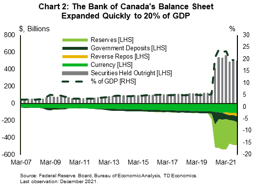
- Since the start of the pandemic central banks have supplemented traditional monetary policy with large-scale asset purchases (aka Quantitative Easing). In Canada and the U.S. central bank balance sheets have expanded by close to 20% of GDP over the past two years.
- Central bank asset purchases were pivotal in calming financial markets during the period of dysfunction in the spring of 2020. Since then QE appears to have had a modest impact in reducing yields.
- With ongoing economic recovery and continued upside inflation surprises, central banks will soon begin reversing course – raising policy rates and normalizing their balance sheets, a process known as Quantitative Tightening (QT).
- QT will reinforce central banks policy hikes and, by increasing the supply of bonds available to the public, put downward pressure on bond prices and upward pressure on yields.
- As central banks allow assets to roll of their balance sheets, reserve balances will decline, putting downward pressure on commercial bank deposits. As long as the process is gradual enough and lending growth remains positive, deposits will decelerate but not shrink outright..
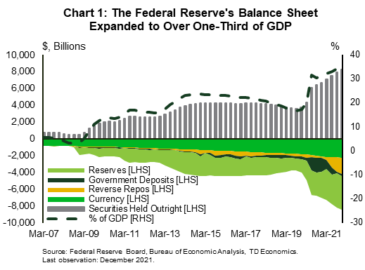
Since the pandemic struck, central banks have been engaging in large scale purchases of government bonds, a process known as quantitative easing (QE). Since 2019, the Federal Reserve’s balance sheet has increased by $4.5 trillion, taking it from 17% of GDP to 35% of GDP (Chart 1). By comparison, the Bank of Canada’s rapid balance sheet expansion amounts to 20% of GDP (Chart 2).
QE’s impact was most significant during the initial lockdown phase of the pandemic in early 2020. It was a clear market signal that injected calm, order and liquidity into the Treasury market during the dash for cash that had pushed up yields on the safest of financial assets. Its subsequent impact on yields appears more modest.
Its impact on commercial bank deposits was more substantive and direct. Central bank purchases of bonds from the private sector directly increased reserves and deposits within the banking sector. Likewise, quantitative tightening (QT) will reduce reserve balances, increase the supply of Treasuries available to the public and put downward pressure on commercial bank deposits.
As was discovered during the Fed’s first foray into QT, unwinding the balance sheet may prove more difficult than expanding it. Due to its interaction with the regulatory environment, reductions in reserves could impose greater funding challenges on the financial sector that augment its impact on the real economy. This augurs for a measured approach. As long as the process is gradual enough and commercial banks continue to lend, deposit growth will decelerate but is unlikely to shrink outright.
QE helped reduce bond yields when policy rates hit zero
Central banks engage in QE to maintain downward pressure on interest rates when they have already taken their policy rate to the effective (zero) lower bound. There are two channels through which QE is thought to impact longer-term yields: the signaling channel and the portfolio balance or preferred habitat channel.
The signaling channel is straightforward and uncontroversial. It relies on the fact that for a risk-free asset, the return to holding a long-term bond to maturity and rolling over a short-term bond over the same period should be roughly the same. Thought of this way, longer-term interest rates reflect investors’ expectations for short-term interest rates plus a risk premium. By reinforcing the central bank’s commitment to maintaining its short-term policy rate at the zero-lower bound, QE lowers expectations for future short-term rates and, therefore, interest rates across the yield curve.
The second “portfolio balance” channel works by reducing the term-premium – the additional return investors require for holding longer term assets. By reducing the supply of assets available to the public, QE raises their price, thereby reducing their yield. This channel interplays with another theoretical concept, which speculates that as long as enough investors have a “preferred habitat” – inelastic demand for assets at specific maturities, the central bank can lower their yields by reducing their supply.
Empirical studies on “portfolio balance” theory suggest that the channel is particularly important in stress periods, like 2008-2009 or March 2020. In normal times, its impact is reduced by rational investors arbitraging it away. That is, if QE pushes bond prices too far out of line with their expected value, non-central bank investors (the majority of the bond market), will sell them and push yields closer to fundamentals. As a result, the consensus among monetary economists is that to the extent QE reduces bond yields, it does so primarily through the signaling mechanism.
Even so, the magnitude of the impact of QE on yields is uncertain. A survey of the literature by Joseph E. Gagnon of the Peterson Institute for International Economics found that asset purchases equivalent to 10% of GDP made in the aftermath of the Global Financial Crisis (GFC), reduced 10-year government bond yields by as much as 240 basis points and as little as 40 basis points, with a median estimate of roughly 50 basis points.1
Given asset purchases worth roughly 20% of GDP during the pandemic, the Gagnon estimate would imply a cumulative reduction in the 10-year yield of roughly 100 basis points. At its lowest point in early 2020, the 10-year yield fell by 120 basis points, but the federal funds rate fell by an even greater 150 basis points. Extracting market expectations for short-term rates from futures markets, the term premium imbedded in the 10-year Treasury declined by just 50 basis points from its level in 2019. Even if all of this decline was due to QE, it would imply a smaller overall impact during the pandemic recession than estimated in the aftermath of the GFC.
This suggests that the QE may exhibit diminished marginal returns. In Canada, the QE announcement of March 27, 2020 carried an element of surprise, as it was not anticipated by market participants nor reflected precedent during the global financial crisis. This may have resulted in a stronger impulse coming from the supply channel. According to a study by the Bank of Canada, Canadian yields declined by an average of 10 basis points due to this round of QE because of dealers’ expectations about current and expected future reduction in bond supply.2
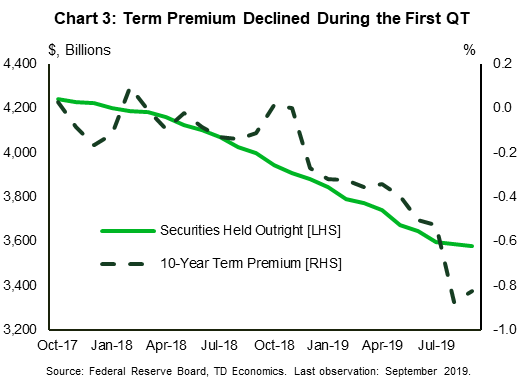
Similar inferences can be drawn on how QT impacts yields. The best example of the signaling mechanism at play is the “taper tantrum” of 2013, when comments by Chair Bernanke resulted in a sell-off in U.S. Treasury bonds. The 10-year yield jumped by 120 basis points between May and August, as investors brought forward their expectations for the timing of policy rate hikes. In contrast, there was little evidence of changes in term premium once the Fed actually initiated QT from 2017 and 2019 (Chart 3).
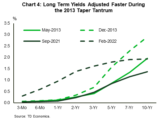
Indeed, anticipation of the end of QE in the here and now appears to have had a relatively limited impact on yields. The 10-year yield has moved by roughly 50 basis points since the Fed began telegraphing its intention to taper asset purchases in September 2021 (Chart 4). Taken together, this suggests that the majority of the change in yields will be the result of changes in expectations for policy rates. Even so, given the large size of central bank balance sheet purchases, even a relatively small impact per dollar of QT could help to lift yields.
The other important difference between QE and QT is that it puts the onus back on the Treasury department to determine the supply of duration to the market. For example, the Treasury may choose to issue more T-bills instead of longer-duration debt. Changes in relatively supply could impact pricing along the yield curve, but this will no longer be the purview of the central bank.
QE creates reserves, QT destroys them, but mind the details
In contrast to its impact on yields, the mechanics of QE on the quantity of reserves is straightforward. When a central bank buys a government bond from a private investor, the proceeds of the purchase are deposited in the banking system. If the seller is a commercial bank with an account at the central bank, the process involves swapping one asset (a government bond) for another (a reserve balance). As reserves can be used immediately for payments, the commercial bank’s balance sheet has been made more liquid, though its overall size is unchanged.
In most cases, the bond is purchased from the public with the commercial bank acting as an intermediary. In this case, the commercial bank’s balance sheet expands – it is credited with a reserve balance on the asset side of its balance sheet and a customer deposit on its liability side.
In its simplest formulation, in which the central bank sells its holdings of bonds, QT is the exact opposite of what’s described above. However, in all likelihood, neither the Federal Reserve nor the Bank of Canada will actively sell its assets, but will simply allow existing bond holdings to mature. The result is the same. Without the central bank purchasing government bonds, the ongoing funding needs of government must be met with additional purchases from the public.
If the new bond buyer is a bank, it will pay for its bond with reserves, which the central bank eliminates with the stroke of a pen. Banks may swap reserves for government debt, but they are unlikely to be the incremental purchasers of additional government bond issuance. In all likelihood, the majority of it will be purchased by a non-bank investors, reducing commercial bank deposits (liabilities) and reserves (assets) just as QE created them.
The devil, however, is in the details. QT interacts with the regulatory environment in a way that may create additional funding needs as deposits run off. Furthermore, differences in the structure of commercial bank balance sheets between Canada and the United States may lead to greater challenges in Canada relative to the United States.
Commercial banks in both Canada and the United States are required to hold enough high-quality liquid assets (HQLA) to fund deposit outflows. This is known as the liquidity coverage ratio (LCR). Prior to the pandemic, LCRs among major banks ranged in the mid 120% range in Canada and the mid 110% in the U.S. With QE increasing reserves and lockdowns impeding economic activity, liquidity coverage ratios rose during the early stages of the pandemic. However, over the course of the past year, lending has rebounded quickly.
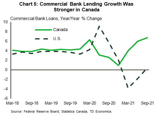
Here the situation differs between Canada and the United States. In Canada, the majority of the pickup in lending has occurred through chartered banks. With lending outpacing deposits, the LCRs of Canadian banks have returned to pre-pandemic levels. In the United States, by contrast, commercial lending growth turned negative in 2021, as PPP loan forgiveness reduced commercial and industrial (C&I) loans and banks packaged their mortgage loans into mortgage backed securities (MBS) and moved them off balance sheet (Chart 5). As a result, LCRs in the U.S. have increased under QE. This is an important distinction. With LCRs back at normal levels in Canada, funding requirements for future lending will be higher in Canada relative to the U.S. As deposits are lost, Canadian banks will have to replace them with other sources of funding in order to maintain LCRs to a greater extent than their American counterparts.
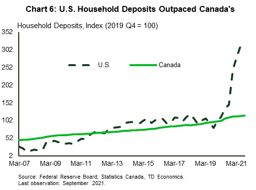
The story does not quite end there. The source of the deposit runoff will also matter. For relatively stable liabilities, such as personal retail deposits, banks are required to hold relatively modest reserves. Both Canada and the United States saw large increases in personal deposits as a result of fiscal transfers and foregone spending during the pandemic. In the U.S., growth in personal deposits has been even stronger than in Canada – the result of more generous fiscal transfers (Chart 6). This creates another source of risk. As these excess personal savings are drawn down, it is likely to result in a shift in the composition of deposits away from personal toward corporate and commercial deposits, which will require more significant levels of reserves, thereby lowering LCRs and increasing funding needs.
Central banks are likely to take a gradual approach to QT
For the reasons above, we expect central banks to take a cautious approach to QT. After all, it is still relatively new. The Federal Reserve only had a brief period to unwind its balance sheet previously before the pandemic hit, which required it to reverse course again. As this was the Bank of Canada’s first foray into QE, it will also be its first into QT.
Second, market dysfunction is more likely to show up as liquidity is withdrawn, relative to when it was added. This was the experience in 2019 when demand for repo financing drove repo rates higher than rates on reserves. In turn, this incented commercial banks to shift reserves into the repo market. This event marked the end of QT as the Fed viewed it as a signal that reserves may have become scarce, even though the overall amount remained large by historical standards (around $1.5 trillion). As a result, the share of assets held by the Fed dropped only marginally, from 22% to 17% of GDP.
Since then, the Fed has implemented a new tool – the Standing Repo Facility (SRF) – where it offers overnight repos each day, allowing money market funds to obtain liquidity directly from the Fed. This helps minimize rate pressures in this market. This, and other facilities, should allow the Fed to maintain control of short-term interest, even while maintaining a large balance sheet.
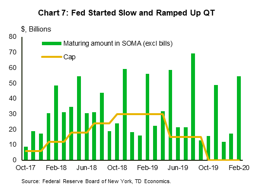
Our baseline expectations for the speed of QT are based on a scaling up of the Fed’s prior attempt. In her press conference in June 2017, four months before the Fed started normalizing its balance sheet for the first time, Chair Janet Yellen stressed that they intended to avoid creating market strains, comparing QT to “watching paint dry.”3 The Fed started QT by limiting the size of U.S. Treasury caps to $6 billion per month, steadily raising the level to $30 billion, before reducing it to $15 billion in 2019 (Chart 7). A similar incrementally larger cap schedule was implemented for agency debt and mortgage-backed securities.
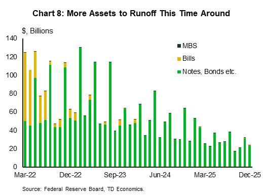
This time, the volume of maturing U.S. Treasury securities is roughly double of that during the previous episode (Chart 8), and so the size of the caps at the peak is likely to be larger. The exact pace of normalization is unknown – the Fed has only released general principles without any details. We assume that the cap will be scaled up by the increase in asset holdings – which would make it roughly $60 billion per month for U.S. Treasuries and $30 billion for MBS. The Fed is likely to start with roughly $10 billion in U.S. Treasuries and $5 billion in MBS per month, building up to $60 and $30 billion respectively over the course of the year.
Once the cap is reached, the ultimate level of reserves is also difficult to know. In 2018, the Fed was estimating that the level of reserves needed was about $600 billion, which would have resulted in reserves dropping to 3% as a share of GDP. Instead, reserves levels came to $1.5 trillion, or roughly 7% of GDP and increased to a maximum of 18% of GDP. We expect the Fed will reduce reserves to reach 7% of GDP (or $1.7 trillion) this time around. This would result in a reserves reduction of roughly $2.1 trillion by the end of 2024. Note that in order to reduce the size of non-Treasury holdings, the Fed will stop reinvesting principal and interest payments into new MBS, effectively letting the current portfolio be repaid. The MBS portfolio will continue to runoff until fully repaid.
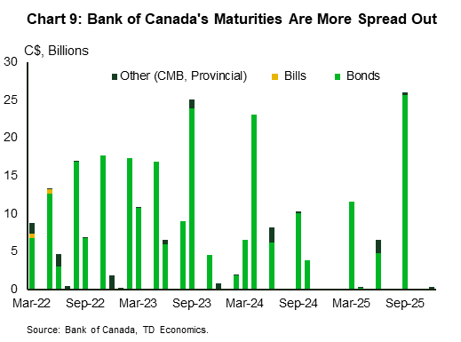
The Bank of Canada’s assets are primarily comprised of government securities whose maturity schedule is more uneven and spread out (Chart 9). We expect that, like the Fed, the Bank of Canada will take a progressive approach, building up its runoff from 15% to 85% of the combined volume of maturing securities.
In the case of Bank of Canada, the amount of QT will depend on whether it wants to go back to its prior system of reserve scarcity, or if it is comfortable continuing to operate policy in a world of abundant reserves. The Bank of Canada has the tools to return to the old system, but we expect it to go slowly, bringing reserve balances from C$270 billion to C$125 billion by the end of 2024.
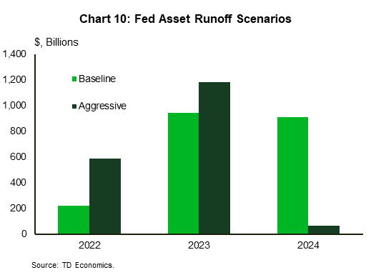
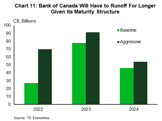
Given considerable uncertainty around the assumptions laid out above, it is worthwhile to examine a more ambitious scenario. A more aggressive central bank strategy would not impose a cap, and to allow for full runoff of their balance sheet based on its average maturity. Assuming the $1.7 trillion level of reserves in the U.S. and outright reserve scarcity in Canada, central banks’ balance sheet normalization of these countries will conclude by early 2024 and early 2026, respectively. In the U.S., the aggressive scenario assumes the same volume of runoff as in baseline – $2.1 trillion – but front-loads it to the earlier year (Chart 10). In Canada, the aggressive scenario is also frontloaded and results in $215 billion of reserves removed by 2024 (Chart 11).
Commercial bank deposits to slow
Under both scenarios, QT puts downward pressure on commercial bank deposits. To the extent that only the public (households and businesses) purchase government bonds, the decline in reserves will match the decline in deposits. However, the impact is unlikely to be one-for-one. As mentioned above, if the banking sector swaps reserves for government securities, there is no change in deposits. Furthermore, central bank’s balance sheet will continue to be impacted by changes in liabilities other than reserves without impacting commercial bank deposits.
For example, incrementally higher supply of U.S. Treasury bills may be absorbed by Money Market funds, which currently hold $1.9 trillion in the Reverse Repo facility (RRP). In the spring of 2021, when the looming debt ceiling forced the Department of Treasury to reduce its deposits at the Fed, while limiting the supply of new Treasury securities, this facility absorbed the extra liquidity. In 2022, Treasury security issuance is expected to increase to offset the reduction in 2021. This will provide users of RRP (Money Market Funds) with the bill supply to swap RRP reserves for Treasuries. These countervailing factors will change the composition of the Fed’s balance sheet, but not impact commercial banks deposits. Canada will experience similar dynamics.
At the same time, deposits will continue to be generated the way they always are, by the extension of loans. This source of money creation is also likely to be impacted by monetary tightening – higher policy rates will reduce demand for loans, but not halt them. In particular, with capacity constraints beginning to bind and government support programs moving to the background, we expect business business lending to continue to perform well over the next several years.
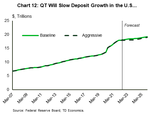
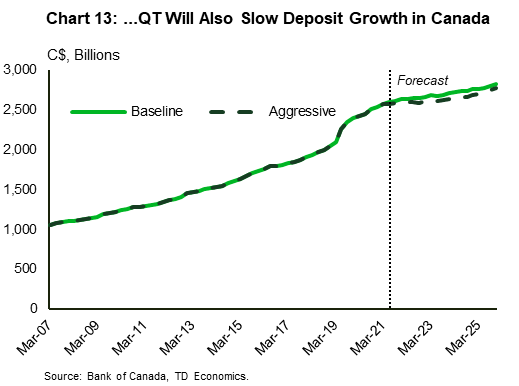
Based on our expectations for loan growth, the baseline QT assumptions outlined above, we expect deposit growth of almost 5% in 2022, to slow to below 2% in 2023 in the United States (Chart 12). In Canada, deposit growth is also expected to slow from 5% in 2022 to under 2% in 2023 (Chart 13).
If central banks choose a more aggressive QT schedule, allowing all their maturing assets to runoff, deposit growth will be even weaker, slowing to a virtual standstill by 2023.
Bottom line
As the economy moves further away from the pandemic shock, central banks are preparing for balance sheet normalization. As a mirror image of QE, QT impacts longer-term yields primarily by signaling higher short-term rates. In practice, these influences are difficult to assess given that markets respond to information in real time with asset repricing occurring long before changes in the balance sheet start to take place.
In contrast to its impact on yields, the mechanics of QT on the quantity of reserves is relatively more straightforward. As a central bank removes assets from its balance sheet, its largest liability (reserves) will also decline. Due to its interaction with liquidity requirements, the downward pressure on deposits may increase funding costs for financial institutions.
This augurs for central banks to go slow. Our baseline expectations for QT in both Canada and the US are based on a gradual ramp up in runoff. We do not expect any active sales of assets, making the length of QT dependent on the level of reserve scarcity – roughly $1.7 trillion in the U.S. and eventually zero in Canada, but not until well into the future..
End Notes
- Gagnon, J. E. “Quantitative Easing: An Underappreciated Success”, Peterson Institute for International Economics. https://www.piie.com/system/files/documents/pb16-4.pdf
- Arora,R., Gungor, S., Nesrallah, J., Ouellet Leblanc, G., Witmer, J. “The impact of the Bank of Canada’s Government Bond Purchase Program”, Bank of Canada. https://www.bankofcanada.ca/2021/10/staff-analytical-note-2021-23/
- See: https://www.federalreserve.gov/mediacenter/files/fomcpresconf20170614.pdf .
Disclaimer
This report is provided by TD Economics. It is for informational and educational purposes only as of the date of writing, and may not be appropriate for other purposes. The views and opinions expressed may change at any time based on market or other conditions and may not come to pass. This material is not intended to be relied upon as investment advice or recommendations, does not constitute a solicitation to buy or sell securities and should not be considered specific legal, investment or tax advice. The report does not provide material information about the business and affairs of TD Bank Group and the members of TD Economics are not spokespersons for TD Bank Group with respect to its business and affairs. The information contained in this report has been drawn from sources believed to be reliable, but is not guaranteed to be accurate or complete. This report contains economic analysis and views, including about future economic and financial markets performance. These are based on certain assumptions and other factors, and are subject to inherent risks and uncertainties. The actual outcome may be materially different. The Toronto-Dominion Bank and its affiliates and related entities that comprise the TD Bank Group are not liable for any errors or omissions in the information, analysis or views contained in this report, or for any loss or damage suffered.
Download
Share: